Electrochemical Impedance Spectroscopy (EIS) Basics

Electrochemical Impedance Spectroscopy (EIS) Basics

1. Introduction

Electrochemical Impedance Spectroscopy (EIS) is a very complex subject in electroanalytical chemistry. This article is designed to help scientists understand what EIS is, how it works, and why EIS is a powerful technique. To understand electrochemical impedance spectroscopy, we will start with the concept of electrical resistance via Ohm’s law (Equation 1), where $\displaystyle{V}$ is the voltage between points (a) and (b), $i$ is the current that flows between (a) and (b), and $R$ is the electrical resistance, represented symbolically by a resistor in as shown in the Figure below. Conceptually, $R$ represents the opposition to the current flowing through an electrical circuit. The larger the $R$ , the less current will flow across the resistor at a given voltage.

$\displaystyle{R=\frac{V}{i}}$

(1)

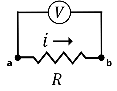
Circuit Diagram of Ohm’s Law. The Voltage (V) is applied between points (a) and (b). The current (i) flows across the resistor (R)

This description of resistance via Ohm’s law applies specifically to direct current (DC), where a static voltage or current is applied across a resistor. Impedance, by contrast, is a measure of the resistance a circuit experiences related to the passage of an alternating electrical current (AC). In an AC system, the applied signal is no longer static but oscillates as a sinusoidal wave at a given frequency. The equation for impedance is analogous to Ohm’s law; however, instead of using $R$ for resistance we use $Z$ for impedance (see Equation 2).

$\displaystyle{Z=\frac{V(\omega)}{i(\omega)}}$

(2)

The impedance $Z$ is proportional to the frequency-dependent voltage $V(\omega)$ and frequency-dependent current $i(\omega)$ , where $\omega$ is the angular frequency of an oscillating sine wave. The definition of impedance comes from electrical circuits, and as a result, voltage is commonly used to define impedance. However, in electrochemical impedance spectroscopy, we will switch from using voltage $V$ to electrical potential, $E$ . Electrical potential is the energy per unit charge gained or lost when current is moved from a known reference point. Voltage represents the difference in potential between two points. For example, in the Figure above, point (a) could have a potential of +100 V and point (b) could have a potential of +101 V with respect to a known reference point, such as ground. In this case, the voltage between (a) and (b) is +1 V. In electrochemical systems, a reference electrode acts as a stable reference point. The potential of the working electrode is measured or applied with respect to the reference electrode potential. There are exceptions to this practice, but in general, the electrochemical potential is used in most electrochemical experiments. For the remainder of this article, the electrical or electrochemical potential will be used when describing EIS.

With a conceptual understanding of impedance, we can look at electrochemical impedance spectroscopy as an electroanalytical technique. In an EIS experiment, a potentiostat applies a sinusoidal potential (or current) signal to an electrochemical system and the resulting current (or potential) signal is recorded and analyzed (see Figure below).

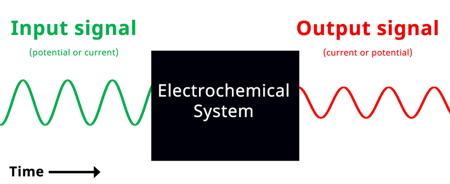
Simplified Electrochemical Impedance Spectroscopy Diagram. If the input signal is potential, then the green wave represents the input sinusoidal potential signal and the red wave represents the output sinusoidal current.

If the applied signal is potential and the measured signal is current, it is referred to as “potentiostatic EIS.” When the applied signal is current and the measured signal is potential, it is referred to as “galvanostatic EIS.” For the case of potentiostatic EIS, a potential is applied with the form shown (Equation 3).

$\displaystyle{E(t)=E_o\cos{(\omega t)}}$

(3)

where $E_o$ is the potential sine wave amplitude, $\omega$ is the angular frequency, $t$ is the time, and the term ${\omega}t$ represents the phase of the waveform. The angular frequency $\omega$ is a measure of how many cycles per unit time the signal oscillates. The amplitude $E_o$ is a measure of the size of the potential or current signal. The user controls the frequency and amplitude of the input potential signal with a potentiostat or frequency response analyzer (FRA). The measured output current signal, $i(t)$ (see Equation 4), has the same frequency as the input signal but its phase may be shifted by a finite amount, known as a phase shift or phase angle, $\phi$ . The measured output current amplitude, $i_o$ , will vary with the impedance of the electrochemical system at a given frequency.

$\displaystyle{i(t)=i_o\cos{(\omega t-\phi)}}$

(4)

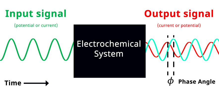
Simplified Electrochemical Impedance Spectroscopy Diagram with Phase Angle. The teal sinusoidal wave represents input potential signal visually overlapped in time with the output current signal. Phase angle represents the shift in phase when the input and output signals are overlapped in time

A complete EIS experiment consists of a sequence of sinusoidal potential signals centered around a potential setpoint. The amplitude of each sinusoidal signal remains constant, but the frequency of the input signal will vary. Typically, frequencies of each input signal are equally spaced on a descending logarithmic scale from ~10 kHz – 1 MHz to a lower limit of ~10 mHz – 1 Hz. For each input potential, a corresponding output current is measured at a given frequency.

Visualization of EIS experiment. The applied input signal and measured output signal have the same frequency. Click to view animation!

The result of plotting the input and output signals on a single current vs. potential graph is called a Lissajous plot (see Figures below). The shape of the current vs. potential Lissajous plot is a straight line (see Figure below) if the input and output signals are in-phase, or if $\phi = 0$ . If the input and output signals are out of phase, the shape of the Lissajous plot appears as a tilted oval (see Figure below). The width of the oval is indicative of the output signal phase angle. For example, if the Lissajous plot looks like a perfect circle, it means the output signal is completely out of phase (i.e., ±90°) with respect to the input signal.

Lissajous plot where the input potential and output current are perfectly in phase. The resulting curve is a straight line with a slope proportional to the impedance at that frequency.

Lissajous plot where the input potential and output current are out of phase. The resulting plot is an oval.

2. Electrochemical Impedance Spectroscopy Data and Plotting

Once the potentiostat collects the potential vs. time and the current vs. time data at each frequency, a Fast Fourier Transform (FFT) is applied to the data. The FFT converts the potential vs. time and current vs. time into potential magnitude vs. frequency and current magnitude vs. frequency.

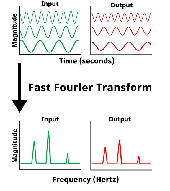
Fast Fourier Transform (FFT) of potential and current vs time data to potential and current magnitude vs frequency data

The potential amplitude ( $E_o$ ), current amplitude ( $i_o$ ), and the phase angle ( $\phi$ ) at each frequency $f$ are determined from the FFT analysis. With these data we can describe the different plotting conventions associated with EIS. The following description simplifies the mathematics, but for a more detailed mathematical description of EIS, check out our Knowledgebase article [*link*].

The magnitude of the impedance is equal to the potential amplitude $E_o$ divided by the current amplitude $i_o$ , as shown in Equation 5.

$\displaystyle{|Z|=\frac{E_o}{i_o}}$

(5)

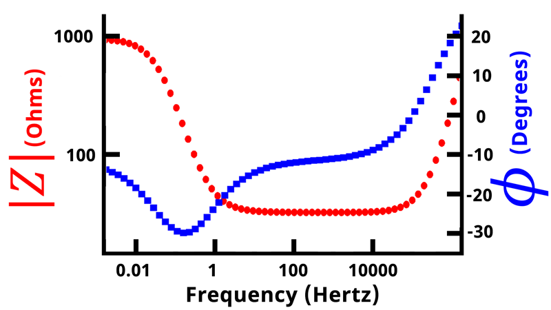
If we plot the magnitude of the impedance $|Z|$ and the phase angle $\phi$ as a function of frequency on a double-axis plot, we get what is called a Bode plot (see Figure below).

Sample Bode Plot

In a Bode plot, $|Z|$ vs. $f$ is displayed on the primary vertical axis and $\phi$ vs. $f$ is displayed on the secondary vertical axis. Frequency and impedance magnitude are normally plotted on a logarithmic scale, while the phase angle is displayed linearly.

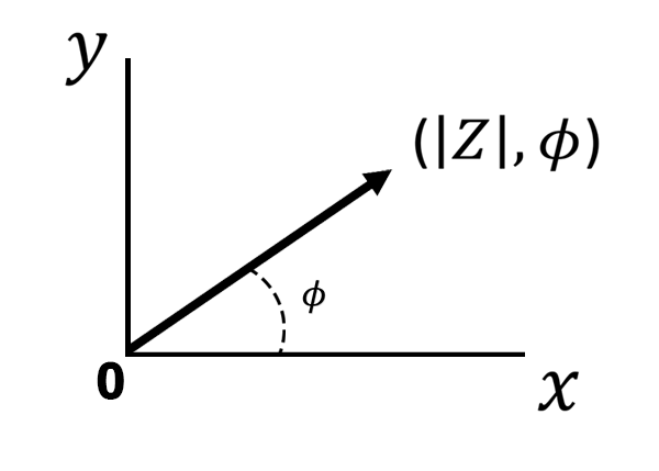
There is another way to express EIS data. Using polar coordinates, let us plot $|Z|$ as a ray originating from the center at an angle equal to the phase angle (see Figure below).

Plotting of Impedance Magnitude and Phase Angle in Polar Coordinates

If we move from polar to cartesian coordinates, we can break the impedance magnitude into its x and y components (see Figure below).

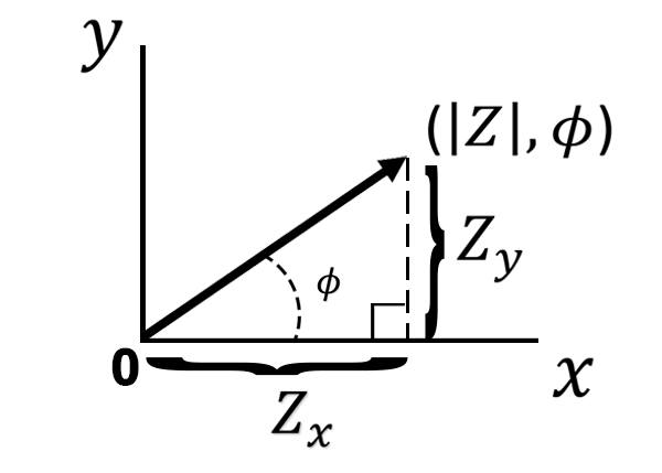
Expressing the Impedance Magnitude in terms of x and y components

Using trigonometry we can describe the impedance of the x-axis $Z_x$ and the impedance of the y-axis $Z_y$ (Equations 6 and Equation 7).

$\displaystyle{Z_x = |Z| \cos{\phi}}$

(6)

$\displaystyle{Z_y = |Z| \sin{\phi}}$

(7)

The $|Z|$ can be described as the vector sum of $Z_x$ and $Z_y$ (Equation 8).

$\displaystyle{|Z| = \sqrt{Z_x^2 + Z_y^2}}$

(8)

The impedance associated with the x-axis is referred to as the real impedance ( $Z_r$ ), and the impedance associated with the y-axis is referred to as the imaginary impedance ( $Z_i$ ). The labels “real” and “imaginary” derive from a more detailed mathematical description of impedance that is beyond the scope of this article. For those interested in a more advanced mathematical derivation, please see this related support article [*link*]. For simplicity, we only need to consider the x-axis component of the impedance magnitude as the real impedance, and the y-axis component of the impedance magnitude as the imaginary impedance. If we plot the real impedance $Z_r$ on the x-axis and the negative imaginary impedance $-Z_i$ on the y-axis we get a Nyquist plot (see Figure below).

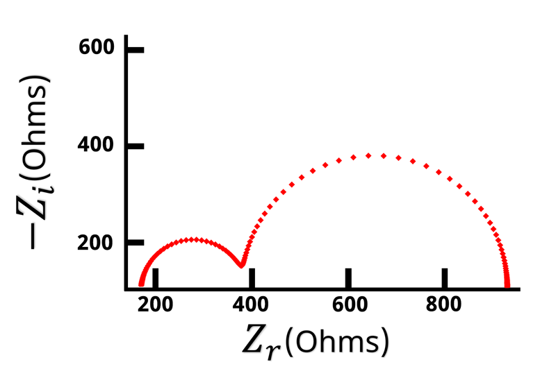
Sample Nyquist Plot

The imaginary impedance values on a Nyquist plot are commonly inverted as shown in the figure above. Alternatively, the $Z_i$ axis is sometimes displayed in reverse numerical order due to the fact that almost all $Z_i$ values are normally less than zero and it is more convenient to view shapes and patterns primarily in the first quadrant on a Cartesian graph (see Figure above). Another convention applied to Nyquist plots is orthonormality, or orthogonality, which refers to the usage of a 1:1 ratio for the visual scale of the x- and y-axes. Note that this does not necessarily mean the numerical scales of the axes need necessarily be identical. One simple way to think of this principle is that when drawing lines on an orthonormal plot around identical values on both axes, it would always make a perfect square (e.g., connect the points (0,0), (0,100), (100,100), and (100,0), and it will be a perfect square).

Nyquist plots are the most common form of displaying impedance data, followed by Bode plots. Bode plots allow easy determination of frequency values, compared with Nyquist plots where frequency values are not plotted. Generally, the lower-leftmost points on a Nyquist plot correspond to the highest frequencies, and following the trace to the right moves from high to low frequency. In total, an electrochemical impedance spectroscopy experiment results in five columns of data: $f$ , $Z_r$ , $Z_i$ , $|Z|$ , and $\phi$ .

3. How to use Electrochemical Impedance Spectroscopy

This section of the article deals with how one models the EIS response with an equivalent circuit and how one solves the model to extract meaningful data from an EIS experiment.

3.1. Circuit Modeling

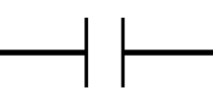
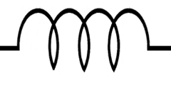
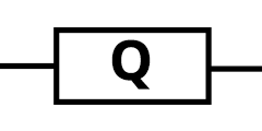
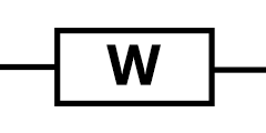
Electrochemical impedance spectroscopy can be used to extract useful information about complex electrochemical systems. The different parts of an electrochemical system can be modeled by known circuit elements, where the impedance is well-characterized. Below you can find a table (see Table below) of known circuit elements and the equations that describes their respective impedances.

Resistor

(R)

Represents electron transfer across an interface

$\displaystyle{Z_R = R}$

Capacitor

(C)

Most often represents non-faradaic charging at an interface

$\displaystyle{Z_C = \frac{1}{j \omega C} = \frac{-j}{\omega C}}$

Inductor

(L)

Represents magnetic inductance

$\displaystyle{Z_L = j \omega L}$

Constant Phase Element

(CPE, Q)

Represents a non-ideal capacitor

$\displaystyle{Z_Q = \frac{1}{{\left (j \omega \right )}^{\alpha} Q}}$

Warburg Element

(W, Ws, Wo)

Represents movement/diffusion of electrons/ions in solid or liquid phases

$\displaystyle{Z_W = \frac{W}{{\left (j \omega \right )}^{0.5}}}$

Gerischer Element

(G)

Represents an electrochemical reaction coupled with an irreversible chemical (irreversible) reaction (may be coupled to diffusion)

$\displaystyle{Z_G = \frac{G}{{\left ( k + j \omega \right )}^{0.5}}}$

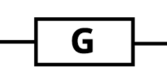
Circuit elements used in EIS modeling.

Note that we use $j$ to indicate the imaginary number $\sqrt{-1}$ . Some textbooks might use $i$ rather than $j$ , but because $i$ normally refers to the current in an electrochemical system, we will be using $j$ .

To understand how we might model an electrochemical system, let us consider a 3-electrode configuration where a conductive working electrode is submerged in an aqueous electrolyte with a redox-active molecule as the analyte (see Figure below). While not shown in this figure, a counter (auxiliary) electrode to maintain charge balance and a reference electrode to act as a stable reference point are implied in the system. The working, counter, and reference electrodes are all connected to a potentiostat. To learn more about how a potentiostat operates in such a configuration, please review our Knowledgebase article on how a potentiostat works.

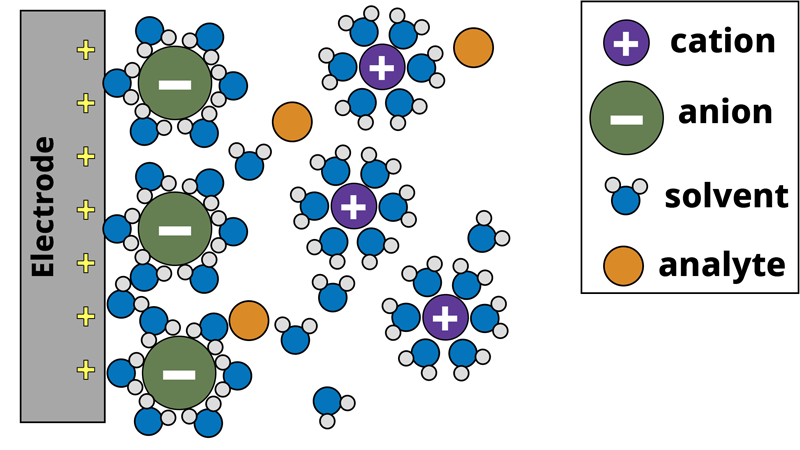
Model of electrode surface in a 3-electrode aqueous system. The gray working electrode applies a positive potential that attracts the negatively charged anions to the surface, forming the electrochemical double-layer.

In the electrochemical system, the potentiostat applies a positive bias to the working electrode with respect to the reference electrode. The positive charge from the working electrode attracts the negatively charged anions to the working electrode surface. The anions are solvated by solvent molecules, and when the anion reaches the electrode surface the solvent molecules surrounding the anion make contact with the electrode surface. This forms a type of capacitor at the electrode surface. A capacitor consists of two oppositely charged plates separated by a dielectric material. In our electrochemical system, the positive charge from the electrode surface is one plate, solvent molecules form the dielectric, and the negatively charged anions form the other plate. This is known as the electrochemical double-layer. The electrochemical system also consists of analyte molecules diffusing around the electrode surface. If we apply a sufficiently positive potential to the working electrode, we can induce an electron transfer (oxidation) from the analyte to the electrode surface. Recall Ohm’s law (Equation 1), where a resistor can be thought of as a measure of the additional potential needed to drive current through a circuit. Similar to Ohm’s law, the electron transfer process can be modeled between the analyte and the electrode as a resistor. Lastly, beyond the electrode surface is the bulk solution where the counter and reference electrodes are located. The electrolyte solution is not a perfect conductor of charge and as such, there is solution resistance between the electrodes as well, which can be modeled as another separate resistor.

At this point, we can construct a simple circuit to describe the electrochemical system. This circuit is commonly used in circuit modeling and is referred to as a Randles circuit (see Figure below),

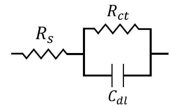
Randles Circuit

where $R_s$ is the solution resistance, $R_{ct}$ is the charge transfer resistance, and $C_{dl}$ is the capacitance of the electrochemical double-layer. We can think of the opposite ends of this circuit as the working and counter electrode, where current flows from the counter electrode (left-hand side) to the working electrode (right-hand side), or vice versa. Visually, you can see that the current has to pass first through the solution resistance $R_s$ . After passing through $R_s$ , however, there exist two possible pathways for the current to flow. It can either move through the capacitor associated with the electrochemical double-layer $C_{dl}$ , or it can pass through the resistor associated with charge transfer $R_{ct}$ . The current will always choose the path of least resistance, or lowest impedance. In this case, the impedance of $C_{dl}$ and $R_{ct}$ vary as a function of frequency.

3.2. Solving the Circuit Model

According to Kirchhoff’s circuit laws, the total impedance of two circuit elements in series is equal to the sum of the two impedances,

$\displaystyle{Z_{\text{series}}=Z_1 + Z_2}$

(9)

Conversely, the reciprocal of the total impedance of two circuit elements in parallel is equal to the sum of the reciprocal of each impedance,

$\displaystyle{\frac{1}{Z_{\text{parallel}}}=\frac{1}{Z_1}+\frac{1}{Z_2}}$

(10)

Equation 10 can be rearranged,

$\displaystyle{Z_{\text{parallel}}=\frac{Z_{1}Z_{2}}{Z_1 + Z_2}}$

(11)

Therefore, the total impedance of our Randles circuit (see Figure above) can be calculated by substituting each circuit element and combining Equation 9, Equation 10, and Equation 11:

$\displaystyle{Z_{Randles}= Z_{R_s}+\frac{Z_{C_{dl}}Z_{R_{ct}}}{Z_{C_{dl}}+Z_{R_{ct}}}}$

(12)

Substituting the respective impedance equations from the Table above for each circuit element results in,

$\displaystyle{Z_{\omega}= R_s+\frac{\frac{R_{ct}}{j\omega C_{dl}}}{R_{ct}+\frac{1}{j\omega C_{dl}}}}$

(13)

After rearranging and simplifying this equation, the impedance of the electrochemical system can be described as

$\displaystyle{Z_{\omega}= R_s+\frac{R_{ct}}{1+R_{ct}C_{dl}(j\omega)}}$

(14)

Remember that $\omega$ is the frequency of our applied potential. When $\omega$ is large or $\omega \rightarrow \infty$ , the denominator becomes very large and the fraction approaches 0. This leaves $Z_{\infty}= R_s$ . While there is no potentiostat that can apply a frequency of $\infty$ Hz, it can often be inferred at the highest frequencies (1 MHz – 100 kHz) that the impedance is equivalent to the solution resistance $R_s$ . At high frequencies the current must travel through the solution resistance, but will then travel through $C_{dl}$ rather than $R_{ct}$ . This is because mathematically as $\omega$ increases, the impedance of the capacitor decreases. You should recall the equation for the impedance of a capacitor from the table above:

$\displaystyle{Z_C = \frac{1}{j\omega C} = \frac{-j}{\omega C}}$

Therefore, at high frequency the capacitor becomes the path of least resistance (see Figure below).

When the frequency of our applied potential is very small, or when $\omega \rightarrow 0$ , the denominator (Equation 14) becomes 1. The impedance therefore reduces to $Z_0= R_s + R_{ct}$ at low frequencies, and the current will travel through $R_{ct}$ rather than $C_{dl}$ . In this case, the impedance of the capacitor $C_{dl}$ becomes very large, and the current will again follow the path of least resistance, which in this case goes through $R_{ct}$ (see Figure below).

Alternative current paths during an EIS experiment. At high frequency, the impedance through the capacitor becomes small, and current travels through the capacitor Cdl. At low frequency, the impedance of the capacitor becomes large and current travels through the resistor Rct.

The Nyquist plot of a Randles circuit can be seen below. When a resistor and capacitor are in parallel, they form a semicircle on the Nyquist plot. Recall that the frequency isn’t directly shown in the Nyquist plot, but typically frequency increases from right to left.

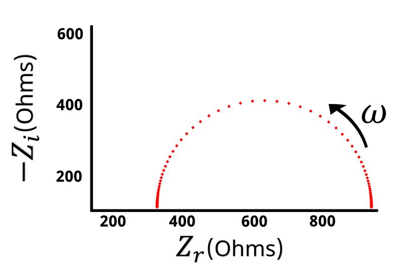
Nyquist plot of Randles Circuit. The frequency typically increases from right to left.

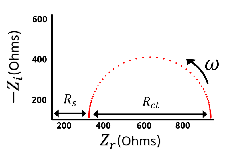
With our understanding of how the impedance behaves at high and low frequencies, values for $R_{ct}$ and $R_s$ can be assigned when looking at the Nyquist plot (see Figure below).

Nyquist plot with R_s and R_ct labeled on the x-axis

Remember that when $\omega$ is large the impedance is equal to $R_s$ . The left hand side of the Nyquist plot represents the high frequency impedance, and the distance from the origin to the high frequency data points is equal to $R_s$ . Conversely, on the opposite side of the semicircle is the low frequency impedance data. When $\omega$ is very low or close to zero, the impedance is equal to $R_s + R_{ct}$ . Based on the high frequency data we know that $R_s$ is the distance from the origin to the left hand side of the semicircle. This means that the width of the semicircle is equal to \displaystyle{R_{ct}}. Looking at the Nyquist plot we can determine the value of $R_s$ and $R_{ct}$ . With $R_s$ and $R_{ct}$ known, we can use Equation 14 to calculate $C_{dl}$ .

The simple Randles circuit above is a fairly common system, but to model more complex electrochemical systems, advanced EIS fitting software is required.

3.3. Why is Electrochemical Impedance Useful?

With a basic understanding of electrochemical impedance spectroscopy, how the technique works, how data is presented, and analyzing EIS data from a simple electrochemical system, the question arises: why use EIS? The double-layer capacitance and solution resistance in an electrochemical system can be determined using DC voltammetry methods. What is special about EIS?

The power of electrochemical impedance spectroscopy is in its ability to probe electrochemical processes on different time scales. This is a unique feature of AC-based electrochemical methods as compared to DC-based electrochemical methods (like cyclic voltammetry). EIS is capable of probing electrochemical processes that might be happening at the same time but on different time scales. For example, the charging of the electrochemical double-layer usually occurs on the microseconds time scale, but diffusion typically occurs on the hundreds of milliseconds time scale. During a DC-based experiment, both processes are happening at the same time and they both contribute to the total current measured. However, it might be difficult to deconvolute the current response from those two processes in a DC-based experiment. EIS, by contrast, can apply a frequency on the time-scale of each process.

The Randles circuit consists of a resistor and a capacitor in parallel, and that circuit is occasionally characterized by its RC time constant. An RC time constant $\tau$ describes how long the capacitor takes to charge up to ~63.2% of its maximum value, or how long it takes to discharge to ~36.8% of its maximum value. Depending on the values of the resistor and capacitor, it could take a long or short time for the capacitor to charge. Electrochemical processes can be thought of in a similar way. Each electrochemical interface, whether it’s a solid/liquid interface or a solid/solid interface can be modeled electrochemically as a Randles or RC circuit. If the time constants of each interface are sufficiently different, then EIS can be used to detect and measure them. If there were multiple electrochemical interfaces in a DC voltammetry experiment, it would be difficult to distinguish between them. That being said, EIS would not be able to easily distinguish between two electrochemical processes with similar values for $\tau$ .

The Randles circuit example in this article is one of the simplest circuit models for an electrochemical system. More complex systems require more complex circuit models. Solving such a circuit model usually requires advanced circuit fitting software and fitting the circuit model provides quantitative information about the electrochemical system. Pine Research Instrumentation offers such software,
and we encourage you to download it and use the built-in circuit fitting tools to analyze your EIS data.

Electrochemical impedance spectroscopy is a complicated electroanalytical chemistry technique. This article serves as an introduction to the technique. There are many other aspects of electrochemical impedance spectroscopy that are not covered in this article; however, some are discussed in other Knowledgebase articles on our website.

4. Related Video

The following YouTube video provides a short introduction to electrochemical impedance spectroscopy, and can be found along with other useful content on the Pine Research YouTube channel.

Help us curate the best support content. Give us a thumbs up if helpful, or a thumbs down if not helpful.

How can we help you today?